plot_precision_recall#
- scikitplot.metrics.plot_precision_recall(y_true, y_probas, *, class_names=None, multi_class=None, class_index=1, to_plot_class_index=None, title='Precision-Recall AUC Curves', ax=None, fig=None, figsize=None, title_fontsize='large', text_fontsize='medium', cmap=None, show_labels=True, digits=4, plot_micro=True, plot_macro=False, pr_auc='pr_auc', ap_score=True, plot_chance_level=True, **kwargs)#
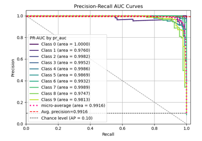
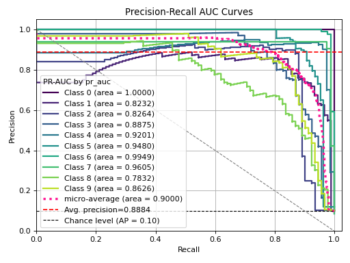
Generates the Precision-Recall AUC Curves from labels and predicted scores/probabilities.
The Precision-Recall curve plots the precision against the recall for different threshold values. The area under the curve (AUC) represents the classifier’s performance. This function supports both binary and multiclass classification tasks.
- Parameters:
y_true (array-like, shape (n_samples,)) – Ground truth (correct) target values.
y_probas (array-like, shape (n_samples,) or (n_samples, n_classes)) – Predicted probabilities for each class or only target class probabilities. If 1D, it is treated as probabilities for the positive class in binary or multiclass classification with the
class_index.class_names (list of str, optional, default=None) – List of class names for the legend. Order should match the order of classes in
y_probas.multi_class ({'ovr', 'multinomial', None}, optional, default=None) – Strategy for handling multiclass classification: - ‘ovr’: One-vs-Rest, plotting binary problems for each class. - ‘multinomial’ or None: Multinomial plot for the entire probability distribution.
class_index (int, optional, default=1) – Index of the class of interest for multi-class classification. Ignored for binary classification.
to_plot_class_index (list-like, optional, default=None) – Specific classes to plot. If a given class does not exist, it will be ignored. If None, all classes are plotted.
title (str, optional, default='Precision-Recall AUC Curves') – Title of the generated plot.
ax (list of matplotlib.axes.Axes, optional, default=None) – The axis to plot the figure on. If None is passed in the current axes will be used (or generated if required). Axes like
fig.add_subplot(1, 1, 1)orplt.gca()fig (matplotlib.pyplot.figure, optional, default: None) –
The figure to plot the Visualizer on. If None is passed in the current plot will be used (or generated if required).
Added in version 0.3.9.
figsize (tuple of int, optional, default=None) – Size of the figure (width, height) in inches.
title_fontsize (str or int, optional, default='large') – Font size for the plot title.
text_fontsize (str or int, optional, default='medium') – Font size for the text in the plot.
cmap (None, str or matplotlib.colors.Colormap, optional, default=None) – Colormap used for plotting. Options include ‘viridis’, ‘PiYG’, ‘plasma’, ‘inferno’, ‘nipy_spectral’, etc. See Matplotlib Colormap documentation for available choices. - https://matplotlib.org/stable/users/explain/colors/index.html - plt.colormaps() - plt.get_cmap() # None == ‘viridis’
show_labels (bool, optional, default=True) – Whether to display the legend labels.
digits (int, optional, default=3) –
Number of digits for formatting PR AUC values in the plot.
Added in version 0.3.9.
plot_micro (bool, optional, default=False) – Whether to plot the micro-average ROC AUC curve.
plot_macro (bool, optional, default=False) – Whether to plot the macro-average ROC AUC curve.
pr_auc ({'average_precision', 'pr_auc'}, optional, default='pr_auc') –
Area under PR AUC curve or Average precision score. sklearn uses default ‘average_precision’ both are slightly different.
Added in version 0.3.9.
ap_score (bool, optional, default: True) –
Annotate the graph with the average precision score, a summary of the plot that is computed as the weighted mean of precisions at each threshold, with the increase in recall from the previous threshold used as the weight.
Added in version 0.3.9.
plot_chance_level (bool, optional, default: True) –
Whether to plot the chance level. The chance level is the prevalence of the positive label. It is used for plotting the chance level line.
Added in version 0.3.9.
- Returns:
The axes with the plotted PR AUC curves.
- Return type:
Notes
The implementation is specific to binary classification. For multiclass problems, the ‘ovr’ or ‘multinomial’ strategies can be used. When
multi_class='ovr', the plot focuses on the specified class (class_index).References#
Examples
>>> from sklearn.datasets import load_digits as data_10_classes
>>> from sklearn.model_selection import train_test_split
>>> from sklearn.naive_bayes import GaussianNB
>>> import scikitplot as skplt
>>> X, y = data_10_classes(return_X_y=True, as_frame=False)
>>> X_train, X_val, y_train, y_val = train_test_split(X, y, test_size=0.5, random_state=0)
>>> model = GaussianNB()
>>> model.fit(X_train, y_train)
>>> y_probas = model.predict_proba(X_val)
>>> skplt.metrics.plot_precision_recall(
>>>     y_val, y_probas,
>>> );
(
Source code,png)