plot_pca_component_variance with examples#

An example showing the plot_pca_component_variance function used by a scikit-learn PCA object.

 # Authors: The scikit-plots developers
 # SPDX-License-Identifier: BSD-3-Clause

Import scikit-plots#

 from sklearn.datasets import (
     load_iris as data_3_classes,
 )
 from sklearn.decomposition import PCA
 from sklearn.model_selection import train_test_split

 import numpy as np

 np.random.seed(0)  # reproducibility
 # importing pylab or pyplot
 import matplotlib.pyplot as plt

 # Import scikit-plot
 import scikitplot as sp

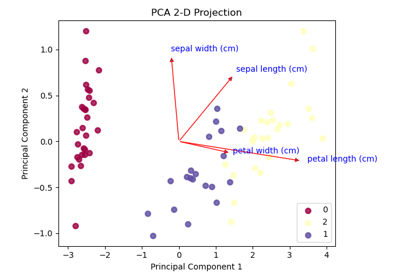
Loading the dataset#

 # Load the data
 X, y = data_3_classes(return_X_y=True, as_frame=False)
 X_train, X_val, y_train, y_val = train_test_split(X, y, test_size=0.5, random_state=0)

PCA#

 # Create an instance of the PCA
 pca = PCA(random_state=0).fit(X_train)

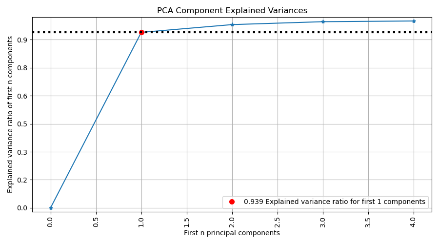
Plot!#

 # Plot!
 ax = sp.decomposition.plot_pca_component_variance(
     pca,
     figsize=(9, 5),
     save_fig=True,
     save_fig_filename="",
     # overwrite=True,
     add_timestamp=True,
     # verbose=True,
 )