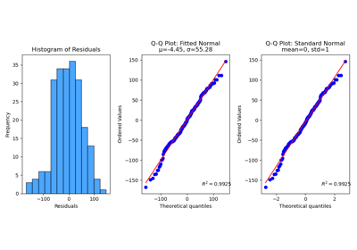
plot_residuals_distribution with examples#
An example showing the plot_residuals_distribution function
with a scikit-learn regressor (e.g., LinearRegression) instance.
# Authors: The scikit-plots developers
# SPDX-License-Identifier: BSD-3-Clause
Import scikit-plots#
from sklearn.datasets import (
    load_diabetes as load_data,
)
from sklearn.linear_model import LinearRegression
from sklearn.model_selection import train_test_split

import numpy as np

np.random.seed(0)  # reproducibility
# importing pylab or pyplot
import matplotlib.pyplot as plt

# Import scikit-plots
import scikitplot as sp
Loading the dataset#
# Load the data
X, y = load_data(return_X_y=True, as_frame=True)
X_train, X_val, y_train, y_val = train_test_split(X, y, test_size=0.5, random_state=0)
Model Training#
# Create an instance of the LogisticRegression
model = LinearRegression().fit(X_train, y_train)

# Perform predictions
y_val_pred = model.predict(X_val)
Plot!#
# Plot!
ax = sp.metrics.plot_residuals_distribution(
    y_val,
    y_val_pred,
    dist_type="normal",
    save_fig=True,
    save_fig_filename="",
    # overwrite=True,
    add_timestamp=True,
    verbose=True,
)
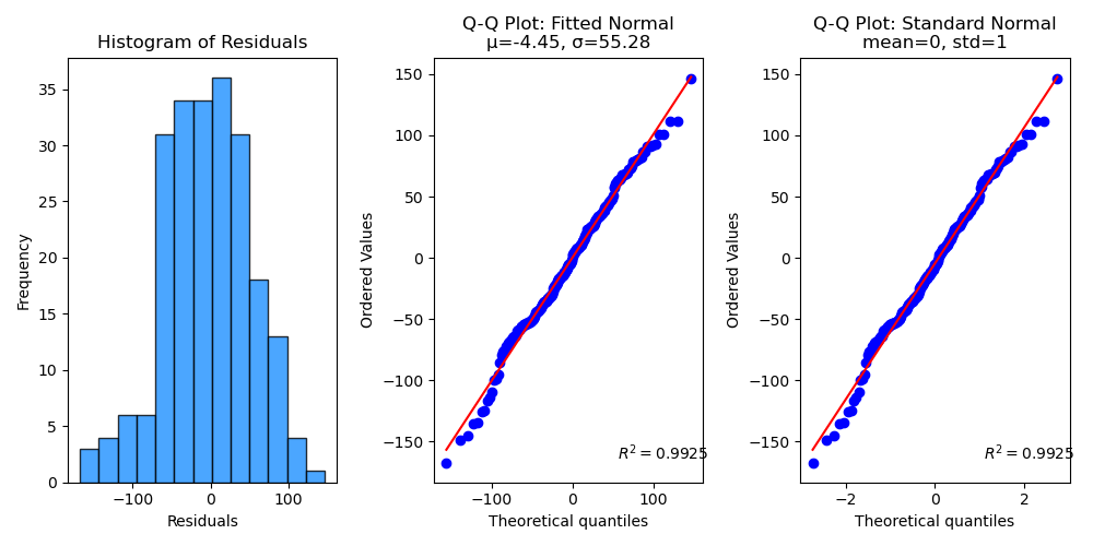
Fitted mean-mu (μ): -4.4509
Fitted std (σ)    : 55.2768
[INFO] Saving path to: /home/circleci/repo/galleries/examples/regression/result_images/plot_residuals_distribution_20260412_091710Z.png
[INFO] Plot saved to: /home/circleci/repo/galleries/examples/regression/result_images/plot_residuals_distribution_20260412_091710Z.png
References
The use of the following functions, methods, classes and modules is shown in this example:
Total running time of the script: (0 minutes 0.789 seconds)
Related examples