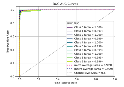
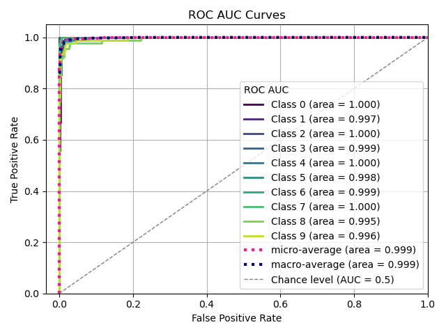
plot_roc_curve with examples#

An example showing the plot_roc_curve function used by a scikit-learn classifier.

# Authors: The scikit-plots developers
# SPDX-License-Identifier: BSD-3-Clause

Import scikit-plots#

from sklearn.datasets import (
    load_digits as data_10_classes,
)
from sklearn.linear_model import LogisticRegression
from sklearn.model_selection import train_test_split

import numpy as np

np.random.seed(0)  # reproducibility
# importing pylab or pyplot
import matplotlib.pyplot as plt

# Import scikit-plot
import scikitplot as sp

Loading the dataset#

# Load the data
X, y = data_10_classes(return_X_y=True, as_frame=False)
X_train, X_val, y_train, y_val = train_test_split(X, y, test_size=0.2, random_state=0)

Model Training#

# Create an instance of the LogisticRegression
model = LogisticRegression(max_iter=1, random_state=0).fit(X_train, y_train)

# Perform predictions
y_val_prob = model.predict_proba(X_val)

/home/circleci/.pyenv/versions/3.11.14/lib/python3.11/site-packages/sklearn/linear_model/_logistic.py:473: ConvergenceWarning:

lbfgs failed to converge after 1 iteration(s) (status=1):
STOP: TOTAL NO. OF ITERATIONS REACHED LIMIT

Increase the number of iterations to improve the convergence (max_iter=1).
You might also want to scale the data as shown in:
    https://scikit-learn.org/stable/modules/preprocessing.html
Please also refer to the documentation for alternative solver options:
    https://scikit-learn.org/stable/modules/linear_model.html#logistic-regression

Plot!#

# Plot!
ax = sp.metrics.plot_roc(
    y_val,
    y_val_prob,
    save_fig=True,
    save_fig_filename="",
    # overwrite=True,
    add_timestamp=True,
    # verbose=True,
)