plot_calibration with examples#
An example showing the plot_calibration function
used by a scikit-learn classifier.
# Authors: The scikit-plots developers
# SPDX-License-Identifier: BSD-3-Clause

# run: Python scripts and shows any outputs directly in the notebook.
# %run ./examples/calibration/plot_calibration_script.py
Import scikit-plots#
from sklearn.calibration import CalibratedClassifierCV
from sklearn.datasets import make_classification
from sklearn.ensemble import RandomForestClassifier
from sklearn.linear_model import LogisticRegression
from sklearn.naive_bayes import GaussianNB
from sklearn.svm import LinearSVC

import numpy as np

np.random.seed(0)  # reproducibility
# importing pylab or pyplot
import matplotlib.pyplot as plt

# Import scikit-plot
import scikitplot as sp
Loading the dataset#
# Load the data
X, y = make_classification(
    n_samples=100000,
    n_features=20,
    n_informative=4,
    n_redundant=2,
    n_repeated=0,
    n_classes=3,
    n_clusters_per_class=2,
    random_state=0,
)
X_train, y_train, X_val, y_val = X[:1000], y[:1000], X[1000:], y[1000:]
Model Training#
# Create an instance of the LogisticRegression
lr_probas = (
    LogisticRegression(max_iter=int(1e5), random_state=0)
    .fit(X_train, y_train)
    .predict_proba(X_val)
)
nb_probas = GaussianNB().fit(X_train, y_train).predict_proba(X_val)
svc_scores = LinearSVC().fit(X_train, y_train).decision_function(X_val)
svc_isotonic = (
    CalibratedClassifierCV(LinearSVC(), cv=2, method="isotonic")
    .fit(X_train, y_train)
    .predict_proba(X_val)
)
svc_sigmoid = (
    CalibratedClassifierCV(LinearSVC(), cv=2, method="sigmoid")
    .fit(X_train, y_train)
    .predict_proba(X_val)
)
rf_probas = (
    RandomForestClassifier(random_state=0).fit(X_train, y_train).predict_proba(X_val)
)

probas_dict = {
    LogisticRegression(): lr_probas,
    # GaussianNB(): nb_probas,
    "LinearSVC() + MinMax": svc_scores,
    "LinearSVC() + Isotonic": svc_isotonic,
    "LinearSVC() + Sigmoid": svc_sigmoid,
    # RandomForestClassifier(): rf_probas,
}
probas_dict
{LogisticRegression(): array([[0.81630981, 0.09296828, 0.09072191],
       [0.67725691, 0.0160746 , 0.30666849],
       [0.25378422, 0.00096865, 0.74524713],
       ...,
       [0.01335815, 0.62376013, 0.36288171],
       [0.03551495, 0.0508954 , 0.91358965],
       [0.00664527, 0.70371215, 0.28964258]], shape=(99000, 3)), 'LinearSVC() + MinMax': array([[ 0.3380658 , -0.70059113, -0.84551216],
       [ 0.32189335, -1.54567754, -0.11575068],
       [ 0.22549259, -2.49509036,  0.69223215],
       ...,
       [-1.4690199 ,  0.16087262, -0.22137806],
       [-1.00072177, -0.95593185,  0.42770417],
       [-1.65162242,  0.34262892, -0.20019956]], shape=(99000, 3)), 'LinearSVC() + Isotonic': array([[0.75192088, 0.18665461, 0.06142451],
       [0.55808311, 0.        , 0.44191689],
       [0.34438275, 0.        , 0.65561725],
       ...,
       [0.01302864, 0.60399643, 0.38297494],
       [0.05420294, 0.10488174, 0.84091532],
       [0.        , 0.58988428, 0.41011572]], shape=(99000, 3)), 'LinearSVC() + Sigmoid': array([[0.73559196, 0.13937371, 0.12503433],
       [0.6086243 , 0.02233023, 0.36904547],
       [0.37500556, 0.00263819, 0.62235624],
       ...,
       [0.02215638, 0.60023759, 0.37760603],
       [0.07558115, 0.1089974 , 0.81542145],
       [0.01489511, 0.64718593, 0.33791896]], shape=(99000, 3))}
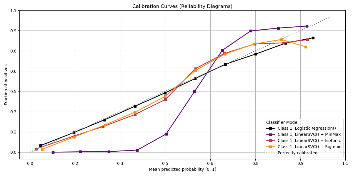
Plot!#
# Plot!
fig, ax = plt.subplots(figsize=(12, 6))
ax = sp.metrics.plot_calibration(
    y_val,
    y_probas_list=probas_dict.values(),
    estimator_names=probas_dict.keys(),
    ax=ax,
    save_fig=True,
    save_fig_filename="",
    overwrite=True,
    add_timestamp=True,
    verbose=True,
)
[INFO] Saving path to: /home/circleci/repo/galleries/examples/calibration/result_images/plot_calibration_20260720_160702Z.png
[INFO] Plot saved to: /home/circleci/repo/galleries/examples/calibration/result_images/plot_calibration_20260720_160702Z.png
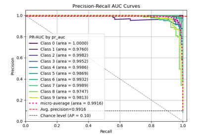
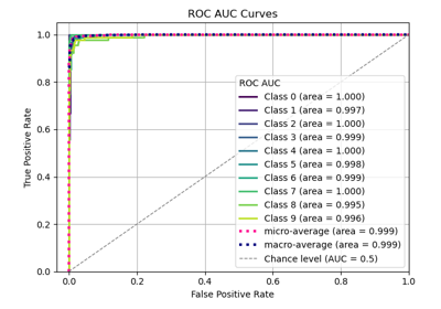
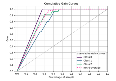
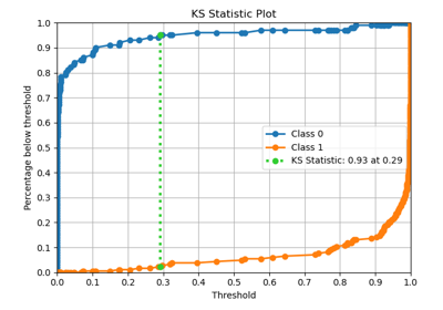
Interpretation
Primary Use: Evaluating probabilistic classifiers by comparing predicted probabilities to observed frequencies of the positive class.
Goal: To assess how well the predicted probabilities align with the actual outcomes, identifying if a model is well-calibrated, overconfident, or underconfident.
Typical Characteristics:
X-axis: Predicted probability (e.g., in bins from 0 to 1).
Y-axis: Observed frequency of the positive class within each bin.
Reference line (diagonal at 45°): Represents perfect calibration, where predicted probabilities match observed frequencies.
Total running time of the script: (0 minutes 2.776 seconds)
Related examples