plot_kdsplot_script with examples

An example showing the kdsplot function used by a scikit-learn regressor.

# Authors: The scikit-plots developers
# SPDX-License-Identifier: BSD-3-Clause

Import scikit-plot

import scikitplot.snsx as sp

import numpy as np; np.random.seed(0)  # reproducibility
import pandas as pd

# Create a DataFrame with predictions
df = pd.DataFrame({
    "y_true": np.random.normal(0.5, 0.1, 100).round(),
    "y_score": np.random.normal(0.5, 0.15, 100),
    "hue": np.random.normal(0.5, 0.4, 100).round(),
})

p = sp.kdsplot(df, x="y_true", y="y_score", kind="df", n_deciles=10, round_digits=2)
p

	decile	prob_min	prob_max	prob_avg	cnt_resp	cnt_resp_total	cnt_resp_non	cnt_resp_wiz	cnt_resp_rndm	rate_resp	cum_resp	cum_resp_pct	cum_resp_total	cum_resp_total_pct	cum_resp_non	cum_resp_non_pct	cum_resp_wiz	cum_resp_wiz_pct	KS	lift
0	1	0.76	0.86	0.79	5.0	10.0	5.0	NaN	5.5	50.0	5.0	9.09	10.0	10.0	5.0	11.11	NaN	NaN	-2.02	0.91
1	2	0.64	0.73	0.68	7.0	10.0	3.0	10.0	5.5	70.0	12.0	21.82	20.0	20.0	8.0	17.78	10.0	18.18	4.04	1.09
2	3	0.60	0.64	0.63	6.0	10.0	4.0	10.0	5.5	60.0	18.0	32.73	30.0	30.0	12.0	26.67	20.0	36.36	6.06	1.09
3	4	0.56	0.60	0.59	9.0	10.0	1.0	10.0	5.5	90.0	27.0	49.09	40.0	40.0	13.0	28.89	30.0	54.55	20.20	1.23
4	5	0.50	0.56	0.53	4.0	10.0	6.0	10.0	5.5	40.0	31.0	56.36	50.0	50.0	19.0	42.22	40.0	72.73	14.14	1.13
5	6	0.45	0.50	0.48	5.0	10.0	5.0	10.0	5.5	50.0	36.0	65.45	60.0	60.0	24.0	53.33	50.0	90.91	12.12	1.09
6	7	0.40	0.44	0.42	4.0	10.0	6.0	5.0	5.5	40.0	40.0	72.73	70.0	70.0	30.0	66.67	55.0	100.00	6.06	1.04
7	8	0.37	0.40	0.39	3.0	10.0	7.0	0.0	5.5	30.0	43.0	78.18	80.0	80.0	37.0	82.22	55.0	100.00	-4.04	0.98
8	9	0.32	0.36	0.34	6.0	10.0	4.0	0.0	5.5	60.0	49.0	89.09	90.0	90.0	41.0	91.11	55.0	100.00	-2.02	0.99
9	10	0.17	0.32	0.28	6.0	10.0	4.0	0.0	5.5	60.0	55.0	100.00	100.0	100.0	45.0	100.00	55.0	100.00	0.00	1.00

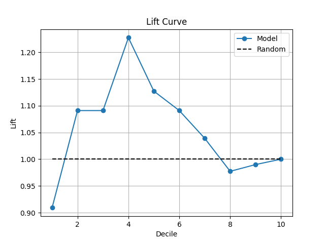
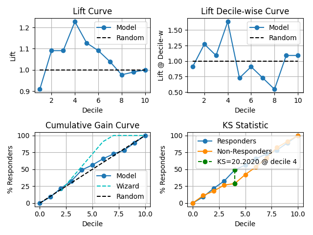
p = sp.kdsplot(df, x="y_true", y="y_score",kind="lift")

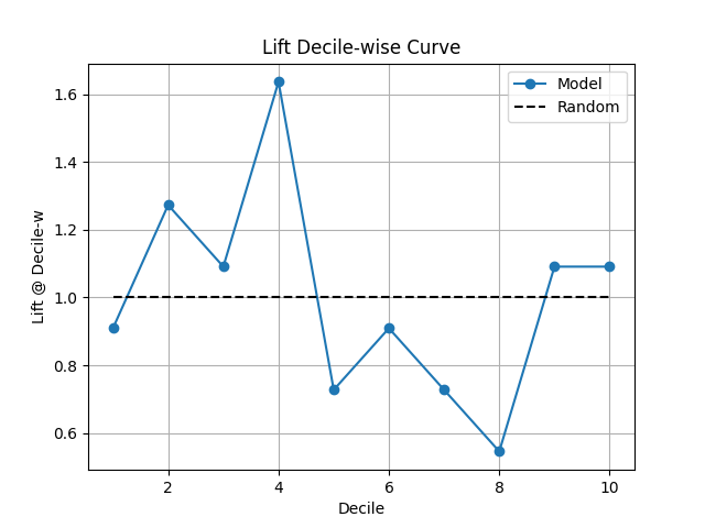
p = sp.kdsplot(df, x="y_true", y="y_score",kind="lift_decile_wise")

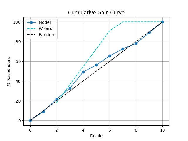
p = sp.kdsplot(df, x="y_true", y="y_score",kind="cumulative_gain")

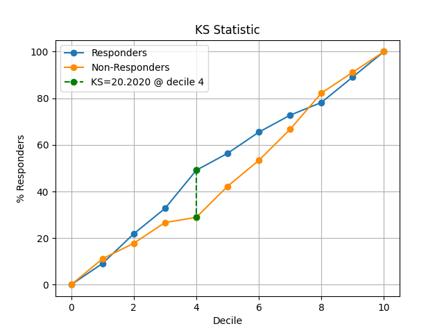
p = sp.kdsplot(df, x="y_true", y="y_score",kind="ks_statistic")

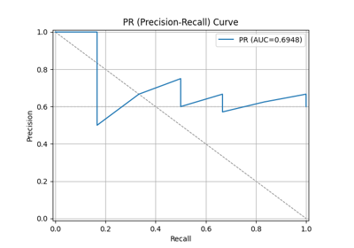
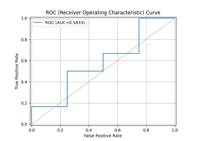
p = sp.kdsplot(df, x="y_true", y="y_score",kind="report", verbose=True)

{
  "decile": "Ranked group (1=highest probability). Why: shows model discrimination. Fatal if top deciles don't capture positives.",
  "prob_min": "Lowest predicted probability in the decile. Why: signals calibration. Fatal if too close to prob_max (model not ranking well).",
  "prob_max": "Highest predicted probability in the decile. Why: checks spread. Fatal if overlaps lower deciles (poor separation).",
  "prob_avg": "Average predicted probability in the decile. Why: good for calibration curves. Fatal if averages do not increase with decile.",
  "cnt_resp": "Number of true responders. Why: measures captured positives. Fatal if counts are flat across deciles (model useless).",
  "cnt_resp_total": "Total samples in the decile. Why: denominator for rates. Fatal if deciles differ in size — signals incorrect binning.",
  "cnt_resp_non": "Number of non-responders. Why: tracks negatives. Fatal if too high in top deciles (bad ranking).",
  "cnt_resp_wiz": "Ideal responders if model was perfect (sorted by actuals). Why: sets maximum benchmark. Fatal if actual is far below this.",
  "cnt_resp_rndm": "Expected responders if random. Why: baseline. Fatal if model only slightly above random.",
  "rate_resp": "Response rate (cnt_resp / total). Why: decile quality. Fatal if early deciles do not outperform later ones.",
  "cum_resp": "Cumulative responders up to decile. Why: shows capture rate. Fatal if curve is too shallow.",
  "cum_resp_pct": "Cumulative responder percentage. Why: needed for lift/gain charts. Fatal if curve near random line.",
  "cum_resp_total": "Cumulative samples. Why: population coverage. Fatal if distribution biased.",
  "cum_resp_total_pct": "Cumulative population percentage. Why: axis for gain/ROC curves. Fatal if deciles unbalanced.",
  "cum_resp_non": "Cumulative non-responders. Why: tracks negatives. Fatal if they dominate early deciles.",
  "cum_resp_non_pct": "Cumulative non-responder %. Why: used in KS. Fatal if almost same as cum_resp_pct (model fails).",
  "cum_resp_wiz": "Cumulative ideal responders. Why: theoretical max. Fatal gap means weak targeting.",
  "cum_resp_wiz_pct": "Cumulative % ideal responders. Why: benchmark. Fatal if actual far below.",
  "KS": "Kolmogorov-Smirnov statistic. Why: measures max separation. Fatal if very low (<0.2). Strong models often 0.3-0.5.",
  "lift": "Cumulative lift vs random. Why: shows model gain. Fatal if <2 in top decile (weak business value)."
}
   decile  prob_min  prob_max  ...  cum_resp_wiz_pct         KS      lift
0       1  0.757001  0.857472  ...               NaN  -2.020202  0.909091
1       2  0.642088  0.731452  ...         18.181818   4.040404  1.090909
2       3  0.602239  0.641672  ...         36.363636   6.060606  1.090909
3       4  0.561119  0.601465  ...         54.545455  20.202020  1.227273
4       5  0.504775  0.559401  ...         72.727273  14.141414  1.127273
5       6  0.446901  0.502622  ...         90.909091  12.121212  1.090909
6       7  0.400478  0.437957  ...        100.000000   6.060606  1.038961
7       8  0.370816  0.398850  ...        100.000000  -4.040404  0.977273
8       9  0.324031  0.363077  ...        100.000000  -2.020202  0.989899
9      10  0.166490  0.316185  ...        100.000000   0.000000  1.000000

[10 rows x 20 columns]

Related examples

plot_prplot_script with examples

plot_prplot_script with examples

plot_rocplot_script with examples

plot_rocplot_script with examples

Visualkeras: Spam Classification Conv1D Dense Example

Visualkeras: Spam Classification Conv1D Dense Example

plot_residuals_distribution with examples

plot_residuals_distribution with examples