plot_calibration#
- scikitplot.api.metrics.plot_calibration(y_true, y_probas_list, *, pos_label=None, class_index=None, class_names=None, to_plot_class_index=1, estimator_names=None, n_bins=10, strategy='uniform', title='Calibration Curves (Reliability Diagrams)', title_fontsize='large', text_fontsize='medium', cmap='inferno', **kwargs)[source]#
Plot calibration curves for a set of classifier probability estimates.
This function plots calibration curves, also known as reliability curves, which are useful to assess the calibration of probabilistic models. For a well-calibrated model, the predicted probability should match the observed frequency of the positive class.
- Parameters:
- y_truearray-like of shape (n_samples,)
Ground truth (correct) target values.
- y_probas_listlist of array-like, shape (n_samples, 2) or (n_samples,)
A list containing the outputs of classifiers’
predict_probaordecision_functionmethods.- n_binsint, optional, default=10
Number of bins to use in the calibration curve. A higher number requires more data to produce reliable results.
- strategystr, optional, default=’uniform’
Strategy used to define the widths of the bins:
‘uniform’: Bins have identical widths.
‘quantile’: Bins have the same number of samples and depend on
y_probas_list.
Added in version 0.3.9.
- estimator_nameslist of str or None, optional, default=None
A list of classifier names corresponding to the probability estimates in
y_probas_list. If None, the names will be generated automatically as “Classifier 1”, “Classifier 2”, etc.- class_nameslist of str or None, optional, default=None
List of class names for the legend. The order should match the classes in
y_probas_list. If None, class indices will be used.- multi_class{‘ovr’, ‘multinomial’, None}, optional, default=None
Strategy for handling multiclass classification: - ‘ovr’: One-vs-Rest, plotting binary problems for each class. - ‘multinomial’ or None: Multinomial plot for the entire probability distribution.
- class_indexint, optional, default=1
Index of the class of interest for multiclass classification. Ignored for binary classification. Related to
multi_classparameter. Not Implemented.- to_plot_class_indexint, list-like, optional, default=1
Specific classes to plot. If a given class does not exist, it will be ignored. If None, all classes are plotted.
- titlestr, optional, default=’Calibration plots (Reliability Curves)’
Title of the generated plot.
- title_fontsizestr or int, optional, default=’large’
Font size of the plot title. Accepts Matplotlib-style sizes like “small”, “medium”, “large”, or an integer.
- text_fontsizestr or int, optional, default=’medium’
Font size of the plot text (axis labels). Accepts Matplotlib-style sizes like “small”, “medium”, “large”, or an integer.
- cmapNone, str or matplotlib.colors.Colormap, optional, default=None
Colormap used for plotting. Options include ‘viridis’, ‘PiYG’, ‘plasma’, ‘inferno’, ‘nipy_spectral’, etc. See Matplotlib Colormap documentation for available choices.
https://matplotlib.org/stable/users/explain/colors/index.html
plt.colormaps()
plt.get_cmap() # None == ‘viridis’
- **kwargs: dict
Generic keyword arguments.
- Returns:
- axmatplotlib.axes.Axes
The axes on which the plot was drawn.
- Other Parameters:
- axmatplotlib.axes.Axes, optional, default=None
The axis to plot the figure on. If None is passed in the current axes will be used (or generated if required).
Added in version 0.4.0.
- figmatplotlib.pyplot.figure, optional, default: None
The figure to plot the Visualizer on. If None is passed in the current plot will be used (or generated if required).
Added in version 0.4.0.
- figsizetuple, optional, default=None
Width, height in inches. Tuple denoting figure size of the plot e.g. (12, 5)
Added in version 0.4.0.
- nrowsint, optional, default=1
Number of rows in the subplot grid.
Added in version 0.4.0.
- ncolsint, optional, default=1
Number of columns in the subplot grid.
Added in version 0.4.0.
- plot_stylestr, optional, default=None
Check available styles with “plt.style.available”. Examples include: [‘ggplot’, ‘seaborn’, ‘bmh’, ‘classic’, ‘dark_background’, ‘fivethirtyeight’, ‘grayscale’, ‘seaborn-bright’, ‘seaborn-colorblind’, ‘seaborn-dark’, ‘seaborn-dark-palette’, ‘tableau-colorblind10’, ‘fast’].
Added in version 0.4.0.
- show_figbool, default=True
Show the plot.
Added in version 0.4.0.
- save_figbool, default=False
Save the plot. Used by
save_plot_decorator.Added in version 0.4.0.
- save_fig_filenamestr, optional, default=’’
Specify the path and filetype to save the plot. If nothing specified, the plot will be saved as png inside
result_imagesunder to the current working directory. Defaults to plot image named to usedfunc.__name__. Used bysave_plot_decorator.Added in version 0.4.0.
- overwritebool, optional, default=True
If False and a file exists, auto-increments the filename to avoid overwriting.
Added in version 0.4.0.
- add_timestampbool, optional, default=False
Whether to append a timestamp to the filename. Default is False.
Added in version 0.4.0.
- verbosebool, optional
If True, enables verbose output with informative messages during execution. Useful for debugging or understanding internal operations such as backend selection, font loading, and file saving status. If False, runs silently unless errors occur.
Default is False.
Added in version 0.4.0: The
verboseparameter was added to control logging and user feedback verbosity.
Notes
The calibration curve is plotted for the class specified by
to_plot_class_index.This function currently supports binary and multiclass classification.
References#
Examples
>>> from sklearn.datasets import make_classification
>>> from sklearn.model_selection import train_test_split
>>> from sklearn.linear_model import LogisticRegression
>>> from sklearn.naive_bayes import GaussianNB
>>> from sklearn.svm import LinearSVC
>>> from sklearn.calibration import CalibratedClassifierCV
>>> from sklearn.ensemble import RandomForestClassifier
>>> from sklearn.model_selection import cross_val_predict
>>> import numpy as np
...
... np.random.seed(0)
>>> # importing pylab or pyplot
>>> import matplotlib.pyplot as plt
>>>
>>> # Import scikit-plot
>>> import scikitplot as skplt
>>>
>>> # Load the data
>>> X, y = make_classification(
>>>     n_samples=100000,
>>>     n_features=20,
>>>     n_informative=4,
>>>     n_redundant=2,
>>>     n_repeated=0,
>>>     n_classes=3,
>>>     n_clusters_per_class=2,
>>>     random_state=0
>>> )
>>> X_train, y_train, X_val, y_val = (
...     X[:1000],
...     y[:1000],
...     X[1000:],
...     y[1000:],
... )
>>>
>>> # Create an instance of the LogisticRegression
>>> lr_probas = (
...     LogisticRegression(max_iter=int(1e5), random_state=0)
...     .fit(X_train, y_train)
...     .predict_proba(X_val)
... )
>>> nb_probas = GaussianNB().fit(X_train, y_train).predict_proba(X_val)
>>> svc_scores = LinearSVC().fit(X_train, y_train).decision_function(X_val)
>>> svc_isotonic = (
...     CalibratedClassifierCV(LinearSVC(), cv=2, method='isotonic')
...     .fit(X_train, y_train)
...     .predict_proba(X_val)
... )
>>> svc_sigmoid = (
...     CalibratedClassifierCV(LinearSVC(), cv=2, method='sigmoid')
...     .fit(X_train, y_train)
...     .predict_proba(X_val)
... )
>>> rf_probas = (
...     RandomForestClassifier(random_state=0)
...     .fit(X_train, y_train)
...     .predict_proba(X_val)
... )
>>>
>>> probas_dict = {
>>>     LogisticRegression(): lr_probas,
>>> # GaussianNB(): nb_probas,
>>>     "LinearSVC() + MinMax": svc_scores,
>>>     "LinearSVC() + Isotonic": svc_isotonic,
>>>     "LinearSVC() + Sigmoid": svc_sigmoid,
>>> # RandomForestClassifier(): rf_probas,
>>> }
>>> # Plot!
>>> fig, ax = plt.subplots(figsize=(12, 6))
>>> ax = skplt.metrics.plot_calibration(
>>>     y_val,
>>>     y_probas_list=probas_dict.values(),
>>>     estimator_names=probas_dict.keys(),
>>>     ax=ax,
>>> );
(
Source code,png)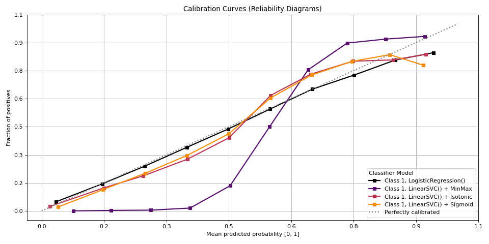