plot_lift

scikitplot.deciles.plot_lift(y_true, y_probas, *, class_names=None, multi_class=None, class_index=1, to_plot_class_index=None, title='Lift Curves', ax=None, fig=None, figsize=None, title_fontsize='large', text_fontsize='medium', cmap=None, show_labels=True, plot_micro=False, plot_macro=False, **kwargs)

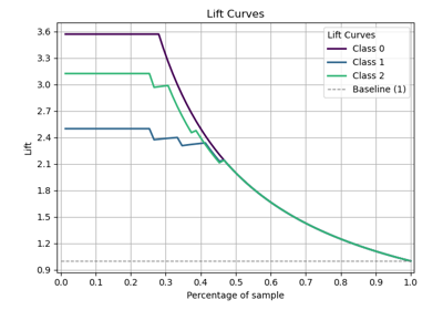
Generate a Lift Curve from true labels and predicted probabilities.

The lift curve evaluates the performance of a classifier by comparing the lift (or improvement) achieved by using the model compared to random guessing. The implementation supports binary classification directly and multiclass classification through One-vs-Rest (OVR) or multinomial strategies.

Parameters:

• y_true (array-like of shape (n_samples,)) – Ground truth (correct) target values.

• y_probas (array-like of shape (n_samples,) or (n_samples, n_classes)) – Predicted probabilities for each class or only target class probabilities. If 1D, it is treated as probabilities for the positive class in binary or multiclass classification with the class_index.

• class_names (list of str, optional, default=None) – List of class names for the legend. Order should match the order of classes in y_probas.

• multi_class ({'ovr', 'multinomial', None}, optional, default=None) – Strategy for handling multiclass classification: - ‘ovr’: One-vs-Rest, plotting binary problems for each class. - ‘multinomial’ or None: Multinomial plot for the entire probability distribution.

• class_index (int, optional, default=1) – Index of the class of interest for multi-class classification. Ignored for binary classification.

• to_plot_class_index (list-like, optional, default=None) – Specific classes to plot. If a given class does not exist, it will be ignored. If None, all classes are plotted. e.g. [0, ‘cold’]

• title (str, default='Lift Curves') – Title of the plot.

• ax (list of matplotlib.axes.Axes, optional, default=None) – The axis to plot the figure on. If None is passed in the current axes will be used (or generated if required). Axes like fig.add_subplot(1, 1, 1) or plt.gca()

• fig (matplotlib.pyplot.figure, optional, default: None) –

  The figure to plot the Visualizer on. If None is passed in the current plot will be used (or generated if required).

  Added in version 0.3.9.

• figsize (tuple of int, optional, default=None) – Size of the figure (width, height) in inches.

• title_fontsize (str or int, optional, default='large') – Font size for the plot title.

• text_fontsize (str or int, optional, default='medium') – Font size for the text in the plot.

• cmap (None, str or matplotlib.colors.Colormap, optional, default=None) – Colormap used for plotting. Options include ‘viridis’, ‘PiYG’, ‘plasma’, ‘inferno’, ‘nipy_spectral’, etc. See Matplotlib Colormap documentation for available choices. - https://matplotlib.org/stable/users/explain/colors/index.html - plt.colormaps() - plt.get_cmap() # None == ‘viridis’

• show_labels (bool, optional, default=True) –

  Whether to display the legend labels.

  Added in version 0.3.9.

• plot_micro (bool, optional, default=False) – Whether to plot the micro-average Lift curve.

• plot_macro (bool, optional, default=False) – Whether to plot the macro-average Lift curve.

• show_labels –

  Whether to display the legend labels.

  Added in version 0.3.9.

Returns:

The axes with the plotted lift curves.

Return type:

matplotlib.axes.Axes

Notes

The implementation is specific to binary classification. For multiclass problems, the ‘ovr’ or ‘multinomial’ strategies can be used. When multi_class='ovr', the plot focuses on the specified class (class_index).

See also

plot_lift_decile_wise

Generates the Decile-wise Lift Plot from labels and probabilities.

References

[1] http://www2.cs.uregina.ca/~dbd/cs831/notes/lift_chart/lift_chart.html

Examples

>>> from sklearn.datasets import load_iris as data_3_classes
>>> from sklearn.model_selection import train_test_split
>>> from sklearn.linear_model import LogisticRegression
>>> import scikitplot as skplt
>>> X, y = data_3_classes(return_X_y=True, as_frame=False)
>>> X_train, X_val, y_train, y_val = train_test_split(X, y, test_size=0.5, random_state=0)
>>> model = LogisticRegression(max_iter=int(1e5), random_state=0).fit(X_train, y_train)
>>> y_probas = model.predict_proba(X_val)
>>> skplt.deciles.plot_lift(
>>>     y_val, y_probas,
>>> );

(Source code, png)

Gallery examples

plot_lift_curve with examples

plot_lift_curve with examples