plot_calibration_curve#
- scikitplot.metrics.plot_calibration_curve(y_true, y_probas_list, y_probas_is_decision, *, n_bins=10, strategy='uniform', estimator_names=None, class_names=None, multi_class=None, class_index=1, to_plot_class_index=[1], title='Calibration Curves (Reliability Diagrams)', ax=None, fig=None, figsize=None, title_fontsize='large', text_fontsize='medium', cmap=None, **kwargs)#
Plot calibration curves for a set of classifier probability estimates.
This function plots calibration curves, also known as reliability curves, which are useful to assess the calibration of probabilistic models. For a well-calibrated model, the predicted probability should match the observed frequency of the positive class.
- Parameters:
y_true (array-like of shape (n_samples,)) – Ground truth (correct) target values.
y_probas_list (list of array-like, shape (n_samples, 2) or (n_samples,)) – A list containing the outputs of classifiers’
predict_probaordecision_functionmethods.y_probas_is_decision (list of bool) – A list indicating whether the classifier’s probability method is
decision_function(True) orpredict_proba(False).n_bins (int, optional, default=10) – Number of bins to use in the calibration curve. A higher number requires more data to produce reliable results.
strategy (str, optional, default='uniform') –
Strategy used to define the widths of the bins: - ‘uniform’: Bins have identical widths. - ‘quantile’: Bins have the same number of samples and depend on
y_probas_list.Added in version 0.3.9.
estimator_names (list of str or None, optional, default=None) – A list of classifier names corresponding to the probability estimates in
y_probas_list. If None, the names will be generated automatically as “Classifier 1”, “Classifier 2”, etc.class_names (list of str or None, optional, default=None) – List of class names for the legend. The order should match the classes in
y_probas_list. If None, class indices will be used.multi_class ({'ovr', 'multinomial', None}, optional, default=None) – Strategy for handling multiclass classification: - ‘ovr’: One-vs-Rest, plotting binary problems for each class. - ‘multinomial’ or None: Multinomial plot for the entire probability distribution.
class_index (int, optional, default=1) – Index of the class of interest for multiclass classification. Ignored for binary classification. Related to
multi_classparameter. Not Implemented.to_plot_class_index (list-like, optional, default=[1]) – Specific classes to plot. If a given class does not exist, it will be ignored. If None, all classes are plotted.
title (str, optional, default='Calibration plots (Reliability Curves)') – Title of the generated plot.
ax (matplotlib.axes.Axes, optional, default=None) – The axis to plot the figure on. If None is passed in the current axes will be used (or generated if required). Axes like
fig.add_subplot(1, 1, 1)orplt.gca()fig (matplotlib.pyplot.figure, optional, default: None) –
The figure to plot the Visualizer on. If None is passed in the current plot will be used (or generated if required).
Added in version 0.3.9.
figsize (tuple, optional) – Tuple denoting the figure size of the plot, e.g., (6, 6). Defaults to
None.title_fontsize (str or int, optional, default='large') – Font size of the plot title. Accepts Matplotlib-style sizes like “small”, “medium”, “large”, or an integer.
text_fontsize (str or int, optional, default='medium') – Font size of the plot text (axis labels). Accepts Matplotlib-style sizes like “small”, “medium”, “large”, or an integer.
cmap (None, str or matplotlib.colors.Colormap, optional, default=None) – Colormap used for plotting. Options include ‘viridis’, ‘PiYG’, ‘plasma’, ‘inferno’, etc. See Matplotlib Colormap documentation for available choices. - https://matplotlib.org/stable/users/explain/colors/index.html
kwargs (dict) – generic keyword arguments.
- Returns:
ax – The axes on which the plot was drawn.
- Return type:
Notes
The calibration curve is plotted for the class specified by
to_plot_class_index.This function currently supports binary and multiclass classification.
References#
Examples
>>> from sklearn.datasets import make_classification
>>> from sklearn.model_selection import train_test_split
>>> from sklearn.linear_model import LogisticRegression
>>> from sklearn.naive_bayes import GaussianNB
>>> from sklearn.svm import LinearSVC
>>> from sklearn.ensemble import RandomForestClassifier
>>> from sklearn.model_selection import cross_val_predict
>>> import numpy as np; np.random.seed(0)
>>>
>>> # Import scikit-plot
>>> import scikitplot as skplt
>>>
>>> # Load the data
>>> X, y = make_classification(
>>>     n_samples=100000,
>>>     n_features=20,
>>>     n_informative=4,
>>>     n_redundant=2,
>>>     n_repeated=0,
>>>     n_classes=3,
>>>     n_clusters_per_class=2,
>>>     random_state=0
>>> )
>>> X_train, y_train, X_val, y_val = X[:1000], y[:1000], X[1000:], y[1000:]
>>>
>>> # Create an instance of the LogisticRegression
>>> lr_probas = LogisticRegression(max_iter=int(1e5), random_state=0).fit(X_train, y_train).predict_proba(X_val)
>>> nb_probas = GaussianNB().fit(X_train, y_train).predict_proba(X_val)
>>> svc_scores = LinearSVC(random_state=0).fit(X_train, y_train).decision_function(X_val)
>>> rf_probas = RandomForestClassifier(random_state=0).fit(X_train, y_train).predict_proba(X_val)
>>>
>>> probas_dict = {
>>>     LogisticRegression(): lr_probas,
>>>     GaussianNB(): nb_probas,
>>>     LinearSVC(): svc_scores,
>>>     RandomForestClassifier(): rf_probas,
>>> }
>>> # Plot!
>>> ax = skplt.metrics.plot_calibration_curve(
>>>     y_val,
>>>     y_probas_list=list(probas_dict.values()),
>>>     estimator_names=list(probas_dict.keys()),
>>>     y_probas_is_decision=list([False, False, True, False]),
>>>     # multi_class='ovr',
>>>     # class_index=1,
>>>     to_plot_class_index=[1],
>>> );
(
Source code,png)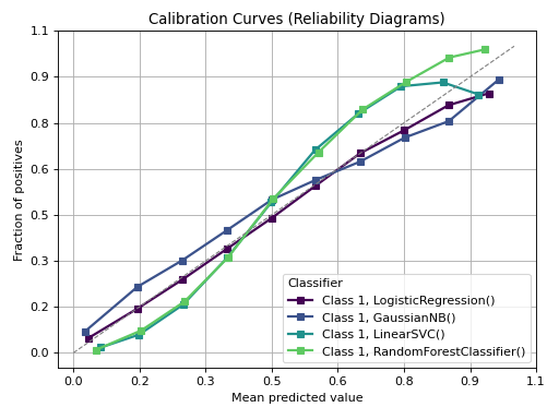