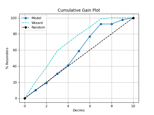
plot_cumulative_gain#
- scikitplot.kds.plot_cumulative_gain(y_true, y_probas, *, pos_label=None, class_index=1, title='Cumulative Gain Plot', title_fontsize='large', text_fontsize='medium', data=None, **kwargs)[source]#
Generates the Decile-wise Lift Plot from labels and probabilities
The lift curve is used to determine the effectiveness of a binary classifier. A detailed explanation can be found at http://www2.cs.uregina.ca/~dbd/cs831/notes/lift_chart/lift_chart.html The implementation here works only for binary classification.
- Parameters:
- y_truearray-like of shape (n_samples,)
Ground truth (correct) target values.
- y_probasarray-like of shape (n_samples,) or (n_samples, n_classes)
Predicted probabilities for each class or only target class probabilities. If 1D, it is treated as probabilities for the positive class in binary or multiclass classification with the
class_index.- class_indexint, optional, default=1
Index of the class of interest for multi-class classification. Ignored for binary classification.
- titlestr, optional, default=’Cumulative Gain Curves’
Title of the generated plot.
- title_fontsizestr or int, optional, default=’large’
Font size for the plot title.
- text_fontsizestr or int, optional, default=’medium’
Font size for the text in the plot.
- **kwargsdict, optional
Generic keyword arguments.
- Returns:
- ax: matplotlib.axes.Axes
The axes with the plotted cumulative gain curves.
- Other Parameters:
- axmatplotlib.axes.Axes, optional, default=None
The axis to plot the figure on. If None is passed in the current axes will be used (or generated if required).
Added in version 0.4.0.
- figmatplotlib.pyplot.figure, optional, default: None
The figure to plot the Visualizer on. If None is passed in the current plot will be used (or generated if required).
Added in version 0.4.0.
- figsizetuple, optional, default=None
Width, height in inches. Tuple denoting figure size of the plot e.g. (12, 5)
Added in version 0.4.0.
- nrowsint, optional, default=1
Number of rows in the subplot grid.
Added in version 0.4.0.
- ncolsint, optional, default=1
Number of columns in the subplot grid.
Added in version 0.4.0.
- plot_stylestr, optional, default=None
Check available styles with “plt.style.available”. Examples include: [‘ggplot’, ‘seaborn’, ‘bmh’, ‘classic’, ‘dark_background’, ‘fivethirtyeight’, ‘grayscale’, ‘seaborn-bright’, ‘seaborn-colorblind’, ‘seaborn-dark’, ‘seaborn-dark-palette’, ‘tableau-colorblind10’, ‘fast’].
Added in version 0.4.0.
- show_figbool, default=True
Show the plot.
Added in version 0.4.0.
- save_figbool, default=False
Save the plot.
Added in version 0.4.0.
- save_fig_filenamestr, optional, default=’’
Specify the path and filetype to save the plot. If nothing specified, the plot will be saved as png inside
result_imagesunder to the current working directory. Defaults to plot image named to usedfunc.__name__.Added in version 0.4.0.
- overwritebool, optional, default=True
If False and a file exists, auto-increments the filename to avoid overwriting.
Added in version 0.4.0.
- add_timestampbool, optional, default=False
Whether to append a timestamp to the filename. Default is False.
Added in version 0.4.0.
- verbosebool, optional
If True, enables verbose output with informative messages during execution. Useful for debugging or understanding internal operations such as backend selection, font loading, and file saving status. If False, runs silently unless errors occur.
Default is False.
Added in version 0.4.0: The
verboseparameter was added to control logging and user feedback verbosity.
See also
print_labelsA legend for the abbreviations of decile table column names.
decile_tableGenerates the Decile Table from labels and probabilities.
plot_liftGenerates the Decile based cumulative Lift Plot from labels and probabilities.
plot_lift_decile_wiseGenerates the Decile-wise Lift Plot from labels and probabilities.
plot_cumulative_gainGenerates the cumulative Gain Plot from labels and probabilities.
plot_ks_statisticGenerates the Kolmogorov-Smirnov (KS) Statistic Plot from labels and probabilities.
Notes
The implementation is specific to binary classification.
References
[1] tensorbored/kds
Examples
>>> from sklearn.datasets import load_iris as data_3_classes
>>> from sklearn.model_selection import train_test_split
>>> from sklearn.linear_model import LogisticRegression
>>> import scikitplot as skplt
>>> X, y = data_3_classes(return_X_y=True, as_frame=False)
>>> X_train, X_val, y_train, y_val = train_test_split(
...     X, y, test_size=0.5, random_state=0
... )
>>> model = LogisticRegression(max_iter=int(1e5), random_state=0).fit(
...     X_train, y_train
... )
>>> y_probas = model.predict_proba(X_val)
>>> skplt.kds.plot_cumulative_gain(
>>>     y_val, y_probas, class_index=1,
>>> );
(
Source code,png)