Gaussian Mixture Models — AIC, AICc, and BIC Model Selection

What is a Gaussian Mixture Model?

Imagine you have a scatter plot of data and you can see a few separate clusters. A Gaussian Mixture Model (GMM) formalises that intuition: it assumes the data came from K overlapping “blobs”, each shaped like a multivariate Gaussian (bell curve). We do not know K ahead of time — that is the whole point of this example.

Mathematically, the model says:

p(x | θ) = Σ_j α_j · N(x | μ_j, Σ_j) for j = 1 … K

where:

K — number of blobs (unknown, to be selected) α_j — how big / common blob j is (all α_j sum to 1) μ_j — centre of blob j Σ_j — shape and orientation of blob j (covariance matrix) θ — shorthand for all of {α_j, μ_j, Σ_j} together

How does sklearn fit the model? (Expectation–Maximisation, EM)

EM is an iterative two-step algorithm:

E-step For each data point, calculate how likely it is that each

blob generated it. These are called “responsibilities”.

M-step Update α, μ, Σ so that the model better explains those

responsibilities.

EM repeats until the improvement per iteration falls below a threshold (tol in sklearn, default 1e-3).

The trouble with just maximising log-likelihood

Adding more blobs always makes the model fit the training data better — it can memorise every point if K is large enough. We need a way to penalise models that are more complex than the data actually warrants. That is what AIC, AICc, and BIC do.

The three criteria

All three are computed from the same two ingredients:

• ln L* the log-likelihood after EM has converged

  (bigger = the model explains the data better)

• p the number of free parameters in the model

  (bigger = the model is more complex)

The formulas:

AIC = -2 ln L* + 2p AICc = -2 ln L* + 2p + 2p(p+1) / (N - p - 1) BIC = -2 ln L* + p · ln N

All three are lower-is-better. The -2 ln L* term rewards a good fit; the second term penalises complexity. The penalties differ:

AIC penalises each parameter by exactly 2. AICc is AIC plus a small extra correction for small sample sizes.

When N is large the correction shrinks to zero and AICc ≈ AIC. When N is small (rough rule: N/p < 40) the correction matters.

BIC penalises each parameter by ln N, which is > 2 for N > 7.

This makes BIC prefer sparser (fewer components) models.

When should I use each?

AIC — your goal is prediction. You are building a generative model

and you want the best out-of-sample log-likelihood. AIC’s softer penalty lets you keep richer structure when the data support it.

AICc — same goal as AIC but your dataset is small or the number of

parameters p is large relative to N. Use AICc by default if you are unsure; for large N it converges to AIC anyway.

BIC — your goal is structure recovery: you want to know the true

number of clusters, not just predict well. BIC’s stronger penalty makes it more likely to land on the right K when one exists. This example uses BIC to pick the final model.

Practical tip: always plot all three. If they all agree on K, you can be confident. If they disagree, the difference is usually just ±1 and you can inspect both models visually.

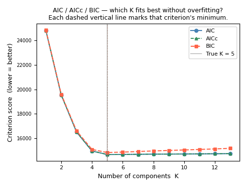
How to read the AIC / AICc / BIC curves

1. Plot score (y-axis) vs K (x-axis).

2. The best K is at the minimum of the curve.

3. A sharp dip → the data strongly prefer that K.

4. A flat plateau → nearby K values are nearly equivalent;

   pick the smaller K (simpler is safer).

5. BIC minimum ≤ AIC minimum — BIC always penalises more, so its minimum shifts left. This is expected, not a bug.

Free parameter count for a full-covariance GMM on d-dimensional data

means : K × d covariances: K × d(d+1)/2 (symmetric matrix, upper triangle only) weights : K - 1 (K weights constrained to sum to 1)

Total p = K × d + K × d(d+1)/2 + (K - 1)

For d=2 (this example): p = 2K + 3K + K - 1 = 6K - 1 For K=5: p = 29

This example

We generate a 2-D dataset from K_true = 5 known Gaussian blobs. Having a ground truth lets us check whether the criteria recover the right K.

Steps:

1. Generate 2 000 points from 5 blobs with different spreads.

2. Fit GMMs for K = 1 … 13.

3. Compute AIC, AICc, and BIC for each K.

4. Pick K_best = argmin(BIC).

5. Produce four plots:

   1. raw 2-D data density (observed histogram)

   2. AIC / AICc / BIC curves with minima marked

   3. best-fit GMM density with component ellipses

   4. side-by-side: observed density vs. recovered density

Dependencies: NumPy, matplotlib, scikit-learn. Nothing else.

References

[1]

Akaike, H. (1974). A new look at the statistical model identification. IEEE Trans. Autom. Control, 19(6), 716-723.

[2]

Schwarz, G. (1978). Estimating the dimension of a model. Ann. Stat., 6(2), 461-464.

[3]

Hurvich, C. M., & Tsai, C.-L. (1989). Regression and time series model selection in small samples. Biometrika, 76(2), 297-307.

[4]

McLachlan, G. J., & Peel, D. (2000). Finite Mixture Models. Wiley-Interscience.

[5]

scikit-learn GaussianMixture docs: https://scikit-learn.org/stable/modules/mixture.html

See Also

sklearn.mixture.GaussianMixture sklearn.datasets.make_blobs

Examples

Run as a standalone script:

python plot_gaussian_mixture_models.py

Import individual helpers inside a notebook:

from plot_gaussian_mixture_models import fit_gmm_range, draw_ellipse

# Authors: The scikit-plots developers
# SPDX-License-Identifier: BSD-3-Clause

Section 1 — Imports

import numpy as np
import matplotlib.pyplot as plt
from matplotlib.patches import Ellipse

from sklearn.datasets import make_blobs
from sklearn.mixture import GaussianMixture

# One seed controls everything: data generation, GMM initialisation,
# and the random-state of all helper functions.
RANDOM_STATE = 42

Section 2 — Utility functions

def _gmm_n_params(k, d, covariance_type="full"):
    """Count the number of free parameters in a fitted GMM.

    This is the ``p`` that goes into AIC, AICc, and BIC.  sklearn computes
    it internally for ``.aic()`` and ``.bic()``; we expose it here so we
    can also compute AICc.

    Parameters
    ----------
    k : int
        Number of Gaussian components.
    d : int
        Number of features (data dimensionality).
    covariance_type : {'full', 'tied', 'diag', 'spherical'}, optional
        Covariance structure.  Default is ``'full'``.

    Returns
    -------
    n_params : int
        Total number of free parameters.

    Notes
    -----
    Breakdown by covariance type (means + covariances + weights):

    full      K*d  +  K*d*(d+1)/2  +  (K-1)   — each component has its
              own full covariance matrix (most expressive, most params).
    tied      K*d  +    d*(d+1)/2  +  (K-1)   — one shared covariance.
    diag      K*d  +          K*d  +  (K-1)   — axis-aligned ellipses.
    spherical K*d  +            K  +  (K-1)   — circular blobs.

    Examples
    --------
    >>> _gmm_n_params(k=5, d=2, covariance_type='full')
    29
    >>> _gmm_n_params(k=5, d=2, covariance_type='diag')
    24
    """
    cov_params = {
        "full":      k * d * (d + 1) // 2,
        "tied":          d * (d + 1) // 2,
        "diag":      k * d,
        "spherical": k,
    }
    if covariance_type not in cov_params:
        raise ValueError(
            f"covariance_type must be one of {list(cov_params)}, "
            f"got '{covariance_type}'."
        )
    return k * d + cov_params[covariance_type] + (k - 1)


def compute_aicc(aic, n_params, n_samples):
    """Compute the corrected AIC (AICc) from a plain AIC value.

    AICc adds a finite-sample correction on top of AIC:

        AICc = AIC + 2p(p+1) / (N - p - 1)

    For large N the correction term shrinks toward zero and AICc ≈ AIC.
    For small N (rough guide: N/p < 40) the correction is meaningful and
    AICc is the safer choice over plain AIC.

    Parameters
    ----------
    aic : float
        Plain AIC value from ``GaussianMixture.aic(X)``.
    n_params : int
        Number of free parameters ``p`` in the model.  Use
        :func:`_gmm_n_params` to compute this.
    n_samples : int
        Number of training data points ``N``.

    Returns
    -------
    aicc : float
        Corrected AIC value.  Returns ``aic`` unchanged when
        ``N - p - 1 <= 0`` (degenerate case; treat result as unreliable).

    Notes
    -----
    The correction term ``2p(p+1)/(N-p-1)`` is always positive, so
    AICc >= AIC.  When N is large the denominator dominates and the
    two values converge.

    Examples
    --------
    >>> compute_aicc(aic=1000.0, n_params=10, n_samples=200)
    1001.1055276381909
    >>> compute_aicc(aic=1000.0, n_params=10, n_samples=10_000)
    1000.02202200220
    """
    denom = n_samples - n_params - 1
    if denom <= 0:
        # N is so small relative to p that the correction is undefined.
        # Return plain AIC and let the caller decide what to do.
        return aic
    return aic + 2.0 * n_params * (n_params + 1) / denom


def draw_ellipse(mean, covariance, ax, n_std=1.5, **kwargs):
    """Draw a confidence ellipse for one 2-D Gaussian component.

    The ellipse captures roughly 74 % of the probability mass for a
    2-D Gaussian when ``n_std=1.5`` (equivalent to a 1.5-sigma contour).

    Internally, we decompose the covariance matrix into eigenvalues and
    eigenvectors.  The eigenvectors tell us the orientation of the ellipse;
    the square-roots of the eigenvalues give the semi-axis lengths.

    Parameters
    ----------
    mean : array-like of shape (2,)
        Centre of the Gaussian component.
    covariance : array-like of shape (2, 2)
        2×2 covariance matrix of the component.
    ax : matplotlib.axes.Axes
        The axes to draw on.
    n_std : float, optional
        Radius of the ellipse in standard deviations.  Default is ``1.5``.
    **kwargs
        Forwarded to ``matplotlib.patches.Ellipse``.  Common ones:
        ``fc`` (face colour), ``ec`` (edge colour), ``lw`` (line width).

    Returns
    -------
    patch : matplotlib.patches.Ellipse
        The patch that was added to *ax*.

    Raises
    ------
    ValueError
        If *covariance* is not exactly 2×2.

    Notes
    -----
    We use ``np.linalg.eigh`` rather than ``eig`` because the covariance
    matrix is always symmetric.  ``eigh`` exploits symmetry for numerical
    stability and guarantees the eigenvalues come back real and sorted.

    Examples
    --------
    >>> import matplotlib.pyplot as plt
    >>> fig, ax = plt.subplots()
    >>> patch = draw_ellipse([0, 0], [[1, 0.5], [0.5, 1]], ax=ax,
    ...                      n_std=2.0, fc='none', ec='black')
    """
    covariance = np.asarray(covariance, dtype=float)
    if covariance.shape != (2, 2):
        raise ValueError(
            f"covariance must be shape (2, 2), got {covariance.shape}."
        )

    # Decompose: eigenvectors = axes directions, eigenvalues = spread along axes
    eigenvalues, eigenvectors = np.linalg.eigh(covariance)

    # Sort largest eigenvalue first (primary axis first)
    order = eigenvalues.argsort()[::-1]
    eigenvalues = eigenvalues[order]
    eigenvectors = eigenvectors[:, order]

    # Angle of the primary axis relative to the x-axis (in degrees)
    angle = np.degrees(np.arctan2(eigenvectors[1, 0], eigenvectors[0, 0]))

    # Full axis lengths = 2 × n_std × sqrt(eigenvalue)
    # np.maximum guards against tiny negative eigenvalues from floating-point
    width  = 2.0 * n_std * np.sqrt(np.maximum(eigenvalues[0], 0.0))
    height = 2.0 * n_std * np.sqrt(np.maximum(eigenvalues[1], 0.0))

    patch = Ellipse(xy=mean, width=width, height=height, angle=angle, **kwargs)
    ax.add_patch(patch)
    return patch


def fit_gmm_range(
    X,
    n_components_range,
    covariance_type="full",
    max_iter=200,
    random_state=None,
):
    """Fit one GMM per value of K and return the models plus AIC, AICc, BIC.

    We loop over every K in *n_components_range*, fit a
    ``GaussianMixture``, and collect AIC, AICc, and BIC.  All models are
    returned so the caller can inspect any of them (not just the best one).

    Parameters
    ----------
    X : array-like of shape (n_samples, n_features)
        Training data.
    n_components_range : array-like of int
        The K values to try, e.g. ``range(1, 14)`` or ``[1, 2, 5, 10]``.
    covariance_type : {'full', 'tied', 'diag', 'spherical'}, optional
        How each component's covariance is parameterised.  ``'full'``
        (default) gives the most flexible shape but uses the most
        parameters — see :func:`_gmm_n_params` for the count.
    max_iter : int, optional
        Hard cap on EM iterations per model.  Default is ``200``.
        Increase if you see ``gmm.converged_ == False`` in practice.
    random_state : int or None, optional
        Seed passed to every ``GaussianMixture`` for reproducibility.
        Default is ``None`` (non-deterministic).

    Returns
    -------
    models : list of GaussianMixture
        One fitted model per K, in the same order as *n_components_range*.
    aic_scores : list of float
        AIC for each model.  Lower is better.
    aicc_scores : list of float
        AICc for each model.  Lower is better.
        Equals AIC for large N; preferred when the dataset is small.
    bic_scores : list of float
        BIC for each model.  Lower is better.

    Raises
    ------
    ValueError
        If *n_components_range* is empty.

    Notes
    -----
    ``init_params='kmeans'`` (sklearn default) is used, which places the
    initial component centres via k-means.  This converges faster and more
    reliably than random initialisation for typical datasets.

    The AICc correction uses the free-parameter count from
    :func:`_gmm_n_params`, which replicates sklearn's internal parameter
    counting.  The three criteria should therefore be mutually consistent.

    Examples
    --------
    >>> import numpy as np
    >>> rng = np.random.default_rng(0)
    >>> X = rng.standard_normal((400, 2))
    >>> models, aic, aicc, bic = fit_gmm_range(X, range(1, 6), random_state=0)
    >>> len(models)
    5
    >>> best_k_bic = np.argmin(bic) + 1
    """
    n_components_range = list(n_components_range)
    if not n_components_range:
        raise ValueError("n_components_range must not be empty.")

    n_samples, n_features = np.asarray(X).shape
    models, aic_scores, aicc_scores, bic_scores = [], [], [], []

    for k in n_components_range:
        gmm = GaussianMixture(
            n_components=k,
            covariance_type=covariance_type,
            max_iter=max_iter,
            random_state=random_state,
        )
        gmm.fit(X)
        models.append(gmm)

        aic_val  = gmm.aic(X)
        bic_val  = gmm.bic(X)
        p        = _gmm_n_params(k, n_features, covariance_type)
        aicc_val = compute_aicc(aic_val, n_params=p, n_samples=n_samples)

        aic_scores.append(aic_val)
        aicc_scores.append(aicc_val)
        bic_scores.append(bic_val)

    return models, aic_scores, aicc_scores, bic_scores


def compute_density_grid(gmm, x_bins, y_bins):
    """Evaluate the log-density of a fitted GMM on a regular 2-D grid.

    We create a meshgrid from *x_bins* and *y_bins*, stack the grid points
    into a (n_points, 2) array, ask the GMM for its log-probability at every
    point, and reshape the result back to (n_y, n_x) so it can be passed
    directly to ``imshow(origin='lower')``.

    Parameters
    ----------
    gmm : GaussianMixture
        A fitted ``GaussianMixture`` instance.
    x_bins : array-like of shape (n_x,)
        x-coordinates of the grid (typically bin centres from a histogram).
    y_bins : array-like of shape (n_y,)
        y-coordinates of the grid.

    Returns
    -------
    log_dens : numpy.ndarray of shape (n_y, n_x)
        Log-probability density at each grid point.
        Pass ``np.exp(log_dens)`` to get plain density for ``imshow``.

    Notes
    -----
    ``score_samples`` returns ``log p(x | θ)`` — the log of the mixture
    density at each point.  We keep it in log space until plotting to
    avoid numerical underflow in sparse regions.

    Examples
    --------
    >>> import numpy as np
    >>> from sklearn.mixture import GaussianMixture
    >>> X = np.random.randn(500, 2)
    >>> gmm = GaussianMixture(n_components=2, random_state=0).fit(X)
    >>> xb = np.linspace(-4, 4, 30)
    >>> yb = np.linspace(-4, 4, 30)
    >>> ld = compute_density_grid(gmm, xb, yb)
    >>> ld.shape
    (30, 30)
    """
    xx, yy = np.meshgrid(x_bins, y_bins)
    X_grid  = np.column_stack([xx.ravel(), yy.ravel()])
    log_dens = gmm.score_samples(X_grid).reshape(len(y_bins), len(x_bins))
    return log_dens


def plot_density_panel(ax, image, extent, label, xlabel="Feature 1",
                       ylabel=None):
    """Show a 2-D density image on *ax* with consistent axes and labelling.

    Parameters
    ----------
    ax : matplotlib.axes.Axes
        The axes to draw on.
    image : numpy.ndarray of shape (n_y, n_x)
        Density values — either raw histogram counts or ``exp(log_dens)``
        from a GMM.
    extent : list of float
        ``[x_min, x_max, y_min, y_max]`` passed directly to ``imshow``.
    label : str
        Short annotation placed in the upper-right corner of the panel.
    xlabel : str, optional
        x-axis label.  Default is ``'Feature 1'``.
    ylabel : str or None, optional
        y-axis label.  Pass ``None`` to omit (useful for right-hand panels
        in a shared-axes layout).

    Returns
    -------
    ax : matplotlib.axes.Axes
        The same axes, modified in place.
    """
    ax.imshow(
        image,
        origin="lower",
        interpolation="nearest",
        aspect="auto",
        extent=extent,
        cmap="binary",
    )
    ax.text(
        0.95, 0.95, label,
        va="top", ha="right",
        transform=ax.transAxes,
        fontsize=9,
    )
    ax.set_xlabel(xlabel, fontsize=9)
    if ylabel is not None:
        ax.set_ylabel(ylabel, fontsize=9)
    ax.tick_params(labelsize=7)
    return ax

Section 3 — Generate synthetic 2-D data

Five blobs with deliberately different spreads (cluster_std). Varying the spreads makes the problem slightly harder and more realistic than equal-variance blobs.

K_TRUE is used only for validation at the end. The GMM fitting loop below never sees this value — it has to figure out K on its own.

K_TRUE   = 5
N_SAMPLES = 2000
N_BINS    = 51

X, y_true = make_blobs(
    n_samples=N_SAMPLES,
    centers=K_TRUE,
    cluster_std=[0.6, 0.8, 0.5, 0.7, 0.9],
    random_state=RANDOM_STATE,
)

Section 4 — Fit GMMs for K = 1 … 13; collect AIC, AICc, BIC

We fit all models upfront so Sections 5–10 are just reads — no recomputation. max_iter=300 is generous for a 2-D problem; lower values are fine too.

N_RANGE = np.arange(1, 14)

models, AIC, AICC, BIC = fit_gmm_range(
    X,
    n_components_range=N_RANGE,
    covariance_type="full",
    max_iter=300,
    random_state=RANDOM_STATE,
)

Section 5 — Pick the best model (minimum BIC)

BIC is preferred here because our goal is recovering the true K, not maximising predictive accuracy. AICc is printed for comparison.

i_best   = int(np.argmin(BIC))
gmm_best = models[i_best]
k_best   = int(N_RANGE[i_best])

print(f"EM converged      : {gmm_best.converged_}")
print(f"BIC-optimal  K    : {k_best}           (true K = {K_TRUE})")
print(f"AIC-optimal  K    : {int(N_RANGE[np.argmin(AIC)])}")
print(f"AICc-optimal K    : {int(N_RANGE[np.argmin(AICC)])}")
print()
print("Scores at BIC-optimal K:")
print(f"  AIC  = {AIC[i_best]:.1f}")
print(f"  AICc = {AICC[i_best]:.1f}  (delta from AIC: {AICC[i_best]-AIC[i_best]:.2f})")
print(f"  BIC  = {BIC[i_best]:.1f}")
print()
n_params_best = _gmm_n_params(k_best, d=2, covariance_type="full")
ratio = N_SAMPLES / n_params_best
print(f"N / p = {N_SAMPLES} / {n_params_best} = {ratio:.1f}")
if ratio < 40:
    print("  → N/p < 40: AICc correction is meaningful here.")
else:
    print("  → N/p >= 40: AICc ≈ AIC for this dataset (correction is tiny).")

EM converged      : True
BIC-optimal  K    : 5           (true K = 5)
AIC-optimal  K    : 5
AICc-optimal K    : 5

Scores at BIC-optimal K:
  AIC  = 14675.3
  AICc = 14676.2  (delta from AIC: 0.88)
  BIC  = 14837.7

N / p = 2000 / 29 = 69.0
  → N/p >= 40: AICc ≈ AIC for this dataset (correction is tiny).

Section 6 — Build observed density (histogram) and GMM density grid

x1_flat = X[:, 0]
x2_flat = X[:, 1]

# np.histogram2d returns counts in H[i, j] = count in bin (x_i, y_j).
# We transpose H before passing to imshow so that rows map to y and
# columns to x, consistent with origin='lower'.
H, x1_edges, x2_edges = np.histogram2d(x1_flat, x2_flat, bins=N_BINS)

x1_centres = 0.5 * (x1_edges[:-1] + x1_edges[1:])
x2_centres = 0.5 * (x2_edges[:-1] + x2_edges[1:])

log_dens = compute_density_grid(gmm_best, x1_centres, x2_centres)

# extent tells imshow the physical coordinate range of the image
extent = [x1_edges[0], x1_edges[-1], x2_edges[0], x2_edges[-1]]

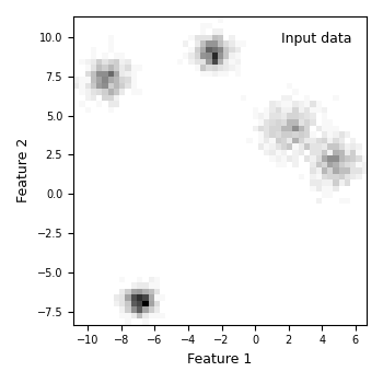
Section 7 — Plot: raw observed density (what the data look like)

This is the “before” panel — purely the data, no model involved.

fig, ax = plt.subplots(figsize=(3.5, 3.5))
plot_density_panel(
    ax,
    image=H.T,
    extent=extent,
    label="Input data",
    xlabel="Feature 1",
    ylabel="Feature 2",
)
fig.tight_layout()
plt.savefig("gmm_01_input_density.png", dpi=150)
plt.show()

Section 8 — Plot: AIC, AICc, and BIC curves

Reading guide (printed in the title too):

• All three curves are lower-is-better.

• The dip / elbow marks the recommended K for each criterion.

• BIC minimum is usually at a smaller K than AIC/AICc — expected.

• AICc ≈ AIC when N is large (lines nearly overlap in that case).

• A flat region means the data cannot distinguish those K values well.

fig, ax = plt.subplots(figsize=(5, 3.8))

ax.plot(N_RANGE, AIC,  "-o",  color="steelblue", markersize=5, label="AIC")
ax.plot(N_RANGE, AICC, "^",   color="seagreen",  markersize=5, label="AICc",
        linestyle=(0, (3, 1, 1, 1)), alpha=0.9)   # dash-dot-dot
ax.plot(N_RANGE, BIC,  "--s", color="tomato",    markersize=5, label="BIC")

# Vertical lines mark each criterion's minimum
k_aic_opt  = int(N_RANGE[np.argmin(AIC)])
k_aicc_opt = int(N_RANGE[np.argmin(AICC)])
k_bic_opt  = k_best

ax.axvline(k_aic_opt,  color="steelblue", lw=0.9, ls=":", alpha=0.8)
ax.axvline(k_aicc_opt, color="seagreen",  lw=0.9, ls=":", alpha=0.8)
ax.axvline(k_bic_opt,  color="tomato",    lw=0.9, ls=":", alpha=0.8)

# Mark the true K with a grey bar so readers can see how close we got
ax.axvline(K_TRUE, color="grey", lw=1.2, ls="-",
           label=f"True K = {K_TRUE}", alpha=0.5)

ax.set_xlabel("Number of components  K", fontsize=9)
ax.set_ylabel("Criterion score  (lower = better)", fontsize=9)
ax.set_title(
    "AIC / AICc / BIC — which K fits best without overfitting?\n"
    "Each dashed vertical line marks that criterion's minimum.",
    fontsize=9,
)
ax.legend(fontsize=8)
ax.tick_params(labelsize=8)
plt.setp(ax.get_yticklabels(), fontsize=7)
fig.tight_layout()
plt.savefig("gmm_02_aic_aicc_bic.png", dpi=150)
plt.show()

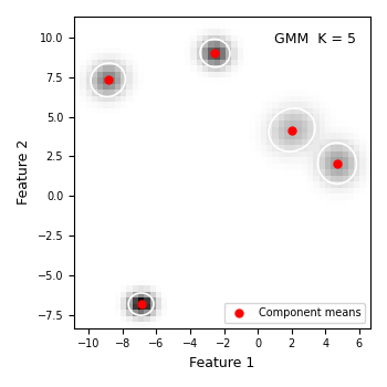
Section 9 — Plot: best-fit GMM density + component ellipses

Each red dot is a component mean. Each white ellipse is the ±1.5σ confidence region of one component — roughly where 74 % of that component’s probability mass sits. If the ellipses align with the visible blobs, the model has captured the data structure well.

fig, ax = plt.subplots(figsize=(3.5, 3.5))
plot_density_panel(
    ax,
    image=np.exp(log_dens),
    extent=extent,
    label=f"GMM  K = {k_best}",
    xlabel="Feature 1",
    ylabel="Feature 2",
)

ax.scatter(
    gmm_best.means_[:, 0],
    gmm_best.means_[:, 1],
    c="red", s=25, zorder=5, label="Component means",
)

for mu, cov in zip(gmm_best.means_, gmm_best.covariances_):
    draw_ellipse(mu, cov, ax=ax, n_std=1.5, fc="none", ec="white", lw=1.2)

ax.legend(fontsize=7, loc="lower right")
fig.tight_layout()
plt.savefig("gmm_03_best_model.png", dpi=150)
plt.show()

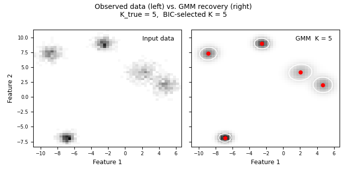
Section 10 — Side-by-side: observed density vs. recovered density

Left panel: the raw data histogram — what we measured. Right panel: the GMM density — what the model learned. Good agreement means the model captured the real structure; systematic differences reveal where the model is wrong.

fig, axes = plt.subplots(1, 2, figsize=(7, 3.5), sharey=True)

plot_density_panel(
    axes[0],
    image=H.T,
    extent=extent,
    label="Input data",
    xlabel="Feature 1",
    ylabel="Feature 2",
)

plot_density_panel(
    axes[1],
    image=np.exp(log_dens),
    extent=extent,
    label=f"GMM  K = {k_best}",
    xlabel="Feature 1",
)

axes[1].scatter(
    gmm_best.means_[:, 0],
    gmm_best.means_[:, 1],
    c="red", s=25, zorder=5,
)
for mu, cov in zip(gmm_best.means_, gmm_best.covariances_):
    draw_ellipse(mu, cov, ax=axes[1], n_std=1.5, fc="none", ec="white", lw=1.2)

fig.suptitle(
    f"Observed data (left) vs. GMM recovery (right)\n"
    f"K_true = {K_TRUE},  BIC-selected K = {k_best}",
    fontsize=10,
)
fig.tight_layout()
plt.savefig("gmm_04_comparison.png", dpi=150)
plt.show()

Tags: model-type: clustering model-workflow: model-selection plot-type: density plot-type: line domain: statistics level: beginner purpose: showcase

Related examples

Memory-Mapping Showcase – Basic / Medium / Advanced

Memory-Mapping Showcase – Basic / Medium / Advanced

Introduction to modelplotpy

Introduction to modelplotpy

Enhanced KISS Random Generator - Complete Usage Examples

Enhanced KISS Random Generator - Complete Usage Examples

Comparing DummyCode Encoder with Other Encoders

Comparing DummyCode Encoder with Other Encoders