plot_pca_2d_projection#

scikitplot.api.decomposition.plot_pca_2d_projection(clf, X, y, *, biplot=False, feature_labels=None, dimensions=[0, 1], label_dots=False, model_type=None, title='PCA 2-D Projection', title_fontsize='large', text_fontsize='medium', cmap='nipy_spectral', **kwargs)[source]#

Plots the 2-dimensional projection of PCA on a given dataset.

Parameters:

clfobject: Fitted PCA instance that can transform given data set into 2 dimensions.
Xarray-like, shape (n_samples, n_features): Feature set to project, where n_samples is the number of samples and n_features is the number of features.
yarray-like, shape (n_samples) or (n_samples, n_features): Target relative to X for labeling.
biplotbool, optional, default=False: If True, the function will generate and plot biplots. If False, the biplots are not generated.
feature_labelsarray-like, shape (n_features), optional, default=None: List of labels that represent each feature of X. Its index position must also be relative to the features. If None is given, labels will be automatically generated for each feature (e.g. “variable1”, “variable2”, “variable3” …).
titlestr, optional, default=’PCA 2-D Projection’: Title of the generated plot.
title_fontsizestr or int, optional, default=’large’: Font size for the plot title.
text_fontsizestr or int, optional, default=’medium’: Font size for the text in the plot.
cmapstr or matplotlib.colors.Colormap, optional, default=’viridis’: Colormap used for plotting the projection. See Matplotlib Colormap documentation for available options: https://matplotlib.org/users/colormaps.html
**kwargs: dict: Generic keyword arguments.

Returns:

axmatplotlib.axes.Axes: The axes on which the plot was drawn.

Other Parameters:

axmatplotlib.axes.Axes, optional, default=None

The axis to plot the figure on. If None is passed in the current axes will be used (or generated if required).

Added in version 0.4.0.

figmatplotlib.pyplot.figure, optional, default: None

The figure to plot the Visualizer on. If None is passed in the current plot will be used (or generated if required).

Added in version 0.4.0.

figsizetuple, optional, default=None

Width, height in inches. Tuple denoting figure size of the plot e.g. (12, 5)

Added in version 0.4.0.

nrowsint, optional, default=1

Number of rows in the subplot grid.

Added in version 0.4.0.

ncolsint, optional, default=1

Number of columns in the subplot grid.

Added in version 0.4.0.

plot_stylestr, optional, default=None

Check available styles with “plt.style.available”. Examples include: [‘ggplot’, ‘seaborn’, ‘bmh’, ‘classic’, ‘dark_background’, ‘fivethirtyeight’, ‘grayscale’, ‘seaborn-bright’, ‘seaborn-colorblind’, ‘seaborn-dark’, ‘seaborn-dark-palette’, ‘tableau-colorblind10’, ‘fast’].

Added in version 0.4.0.

show_figbool, default=True

Show the plot.

Added in version 0.4.0.

save_figbool, default=False

Save the plot.

Added in version 0.4.0.

save_fig_filenamestr, optional, default=’’

Specify the path and filetype to save the plot. If nothing specified, the plot will be saved as png inside result_images under to the current working directory. Defaults to plot image named to used func.__name__.

Added in version 0.4.0.

overwritebool, optional, default=True

If False and a file exists, auto-increments the filename to avoid overwriting.

Added in version 0.4.0.

add_timestampbool, optional, default=False

Whether to append a timestamp to the filename. Default is False.

Added in version 0.4.0.

verbosebool, optional

If True, enables verbose output with informative messages during execution. Useful for debugging or understanding internal operations such as backend selection, font loading, and file saving status. If False, runs silently unless errors occur.

Default is False.

Added in version 0.4.0: The verbose parameter was added to control logging and user feedback verbosity.

Examples

>>> from sklearn.decomposition import PCA
>>> from sklearn.datasets import load_iris as data_3_classes
>>> import scikitplot as skplt
>>> X, y = data_3_classes(return_X_y=True, as_frame=True)
>>> pca = PCA(random_state=0).fit(X)
>>> skplt.decomposition.plot_pca_2d_projection(
...     pca,
...     X,
...     y,
...     biplot=True,
...     feature_labels=X.columns.tolist(),
... )

(Source code, png)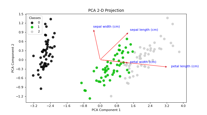

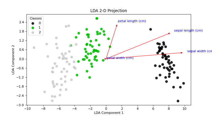
>>> from sklearn.discriminant_analysis import (
...     LinearDiscriminantAnalysis,
... )
>>> from sklearn.datasets import load_iris as data_3_classes
>>> import scikitplot as skplt
>>> X, y = data_3_classes(return_X_y=True, as_frame=True)
>>> clf = LinearDiscriminantAnalysis().fit(X, y)
>>> skplt.decomposition.plot_pca_2d_projection(
...     clf,
...     X,
...     y,
...     biplot=True,
...     feature_labels=X.columns.tolist(),
... )

(Source code, png)

plot_pca_2d_projection#

This Page