plot_classifier_eval#
- scikitplot.api.metrics.plot_classifier_eval(y_true, y_pred, *, labels=None, normalize=None, digits=3, title='train', title_fontsize='large', text_fontsize='medium', cmap=None, x_tick_rotation=0, figsize=(8, 3), nrows=1, ncols=2, index=2, **kwargs)[source]#
Generates various evaluation plots for a classifier, including confusion matrix, precision-recall curve, and ROC curve.
This function provides a comprehensive view of a classifier’s performance through multiple plots, helping in the assessment of its effectiveness and areas for improvement.
- Parameters:
- y_truearray-like, shape (n_samples,)
Ground truth (correct) target values.
- y_predarray-like, shape (n_samples,)
Predicted target values from the classifier.
- labelslist of string, optional
List of labels for the classes. If None, labels are automatically generated based on the class indices.
- normalize{‘true’, ‘pred’, ‘all’, None}, optional
Normalizes the confusion matrix according to the specified mode. Defaults to None.
‘true’: Normalizes by true (actual) values.
‘pred’: Normalizes by predicted values.
‘all’: Normalizes by total values.
None: No normalization.
- digitsint, optional, default=3
Number of digits for formatting floating point values in the plots.
- titlestring, optional, default=’train’
Title of the generated plot.
- title_fontsizestring or int, optional, default=”large”
Font size for the plot title. Use e.g. “small”, “medium”, “large” or integer values.
- text_fontsizestring or int, optional, default=”medium”
Font size for the text in the plot. Use e.g. “small”, “medium”, “large” or integer values.
- cmapNone, str or matplotlib.colors.Colormap, optional, default=None
Colormap used for plotting. Options include ‘viridis’, ‘PiYG’, ‘plasma’, ‘inferno’, ‘nipy_spectral’, etc. See Matplotlib Colormap documentation for available choices.
https://matplotlib.org/stable/users/explain/colors/index.html
plt.colormaps()
plt.get_cmap() # None == ‘viridis’
- x_tick_rotationint, optional, default=0
Rotates x-axis tick labels by the specified angle.
Added in version 0.3.9.
- **kwargs: dict
Generic keyword arguments.
- Returns:
- figmatplotlib.figure.Figure
The figure on which the plot was drawn.
- Other Parameters:
- axmatplotlib.axes.Axes, optional, default=None
The axis to plot the figure on. If None is passed in the current axes will be used (or generated if required).
Added in version 0.4.0.
- figmatplotlib.pyplot.figure, optional, default: None
The figure to plot the Visualizer on. If None is passed in the current plot will be used (or generated if required).
Added in version 0.4.0.
- figsizetuple, optional, default=None
Width, height in inches. Tuple denoting figure size of the plot e.g. (12, 5)
Added in version 0.4.0.
- nrowsint, optional, default=1
Number of rows in the subplot grid.
Added in version 0.4.0.
- ncolsint, optional, default=1
Number of columns in the subplot grid.
Added in version 0.4.0.
- plot_stylestr, optional, default=None
Check available styles with “plt.style.available”. Examples include: [‘ggplot’, ‘seaborn’, ‘bmh’, ‘classic’, ‘dark_background’, ‘fivethirtyeight’, ‘grayscale’, ‘seaborn-bright’, ‘seaborn-colorblind’, ‘seaborn-dark’, ‘seaborn-dark-palette’, ‘tableau-colorblind10’, ‘fast’].
Added in version 0.4.0.
- show_figbool, default=True
Show the plot.
Added in version 0.4.0.
- save_figbool, default=False
Save the plot. Used by
save_plot_decorator.Added in version 0.4.0.
- save_fig_filenamestr, optional, default=’’
Specify the path and filetype to save the plot. If nothing specified, the plot will be saved as png inside
result_imagesunder to the current working directory. Defaults to plot image named to usedfunc.__name__. Used bysave_plot_decorator.Added in version 0.4.0.
- overwritebool, optional, default=True
If False and a file exists, auto-increments the filename to avoid overwriting.
Added in version 0.4.0.
- add_timestampbool, optional, default=False
Whether to append a timestamp to the filename. Default is False.
Added in version 0.4.0.
- verbosebool, optional
If True, enables verbose output with informative messages during execution. Useful for debugging or understanding internal operations such as backend selection, font loading, and file saving status. If False, runs silently unless errors occur.
Default is False.
Added in version 0.4.0: The
verboseparameter was added to control logging and user feedback verbosity.
Notes
The function generates and displays multiple evaluation plots. Ensure that
y_trueandy_predhave the same shape and contain valid class labels. Thenormalizeparameter is applicable to the confusion matrix plot. Adjustcmapandx_tick_rotationto customize the appearance of the plots.Examples
>>> from sklearn.datasets import load_digits as data_10_classes
>>> from sklearn.model_selection import train_test_split
>>> from sklearn.naive_bayes import GaussianNB
>>> import scikitplot as skplt
>>> X, y = data_10_classes(return_X_y=True, as_frame=False)
>>> X_train, X_val, y_train, y_val = train_test_split(X, y, test_size=0.5, random_state=0)
>>> model = GaussianNB()
>>> model.fit(X_train, y_train)
>>> y_val_pred = model.predict(X_val)
>>> skplt.metrics.plot_classifier_eval(
>>>     y_val, y_val_pred,
>>>     title='val',
>>> );
(
Source code,png)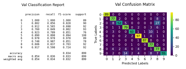