plot_precision_recall#
- scikitplot.api.metrics.plot_precision_recall(y_true, y_probas, *, class_index=None, class_names=None, multi_class=None, to_plot_class_index=None, title='Precision-Recall AUC Curves', title_fontsize='large', text_fontsize='medium', cmap=None, show_labels=True, digits=4, plot_micro=True, plot_macro=False, pr_auc='pr_auc', ap_score=True, plot_chance_level=True, **kwargs)[source]#
Generates the Precision-Recall AUC Curves from labels and predicted scores/probabilities.
Precision-Recall curve plots the precision against the recall for different threshold values. The area under the curve (AUC) represents the classifier’s performance. This function supports both binary and multiclass classification tasks.
- Parameters:
- y_truearray-like, shape (n_samples,)
Ground truth (correct) target values.
- y_probasarray-like, shape (n_samples,) or (n_samples, n_classes)
Predicted probabilities for each class or only target class probabilities. If 1D, it is treated as probabilities for the positive class in binary or multiclass classification with the
class_index.- class_nameslist of str, optional, default=None
List of class names for the legend. Order should match the order of classes in
y_probas.- multi_class{‘ovr’, ‘multinomial’, None}, optional, default=None
Strategy for handling multiclass classification:
‘ovr’: One-vs-Rest, plotting binary problems for each class.
‘multinomial’ or None: Multinomial plot for the entire probability distribution.
- class_indexint, optional, default=1
Index of the class of interest for multi-class classification. Ignored for binary classification.
- to_plot_class_indexlist-like, optional, default=None
Specific classes to plot. If a given class does not exist, it will be ignored. If None, all classes are plotted.
- titlestr, optional, default=’Precision-Recall AUC Curves’
Title of the generated plot.
- title_fontsizestr or int, optional, default=’large’
Font size for the plot title.
- text_fontsizestr or int, optional, default=’medium’
Font size for the text in the plot.
- cmapNone, str or matplotlib.colors.Colormap, optional, default=None
Colormap used for plotting. Options include ‘viridis’, ‘PiYG’, ‘plasma’, ‘inferno’, ‘nipy_spectral’, etc. See Matplotlib Colormap documentation for available choices.
https://matplotlib.org/stable/users/explain/colors/index.html
plt.colormaps()
plt.get_cmap() # None == ‘viridis’
- show_labelsbool, optional, default=True
Whether to display the legend labels.
- digitsint, optional, default=3
Number of digits for formatting PR AUC values in the plot.
Added in version 0.3.9.
- plot_microbool, optional, default=False
Whether to plot the micro-average ROC AUC curve.
- plot_macrobool, optional, default=False
Whether to plot the macro-average ROC AUC curve.
- pr_auc{‘average_precision’, ‘pr_auc’}, optional, default=’pr_auc’
Area under PR AUC curve or Average precision score. sklearn uses default ‘average_precision’ both are slightly different.
Added in version 0.3.9.
- ap_scorebool, optional, default: True
Annotate the graph with the average precision score, a summary of the plot that is computed as the weighted mean of precisions at each threshold, with the increase in recall from the previous threshold used as the weight.
Added in version 0.3.9.
- plot_chance_levelbool, optional, default: True
Whether to plot the chance level. The chance level is the prevalence of the positive label. It is used for plotting the chance level line.
Added in version 0.3.9.
- **kwargs: dict
Generic keyword arguments.
- Returns:
- matplotlib.axes.Axes
The axes with the plotted PR AUC curves.
- Other Parameters:
- axmatplotlib.axes.Axes, optional, default=None
The axis to plot the figure on. If None is passed in the current axes will be used (or generated if required).
Added in version 0.4.0.
- figmatplotlib.pyplot.figure, optional, default: None
The figure to plot the Visualizer on. If None is passed in the current plot will be used (or generated if required).
Added in version 0.4.0.
- figsizetuple, optional, default=None
Width, height in inches. Tuple denoting figure size of the plot e.g. (12, 5)
Added in version 0.4.0.
- nrowsint, optional, default=1
Number of rows in the subplot grid.
Added in version 0.4.0.
- ncolsint, optional, default=1
Number of columns in the subplot grid.
Added in version 0.4.0.
- plot_stylestr, optional, default=None
Check available styles with “plt.style.available”. Examples include: [‘ggplot’, ‘seaborn’, ‘bmh’, ‘classic’, ‘dark_background’, ‘fivethirtyeight’, ‘grayscale’, ‘seaborn-bright’, ‘seaborn-colorblind’, ‘seaborn-dark’, ‘seaborn-dark-palette’, ‘tableau-colorblind10’, ‘fast’].
Added in version 0.4.0.
- show_figbool, default=True
Show the plot.
Added in version 0.4.0.
- save_figbool, default=False
Save the plot. Used by
save_plot_decorator.Added in version 0.4.0.
- save_fig_filenamestr, optional, default=’’
Specify the path and filetype to save the plot. If nothing specified, the plot will be saved as png inside
result_imagesunder to the current working directory. Defaults to plot image named to usedfunc.__name__. Used bysave_plot_decorator.Added in version 0.4.0.
- overwritebool, optional, default=True
If False and a file exists, auto-increments the filename to avoid overwriting.
Added in version 0.4.0.
- add_timestampbool, optional, default=False
Whether to append a timestamp to the filename. Default is False.
Added in version 0.4.0.
- verbosebool, optional
If True, enables verbose output with informative messages during execution. Useful for debugging or understanding internal operations such as backend selection, font loading, and file saving status. If False, runs silently unless errors occur.
Default is False.
Added in version 0.4.0: The
verboseparameter was added to control logging and user feedback verbosity.
Notes
The implementation is specific to binary classification. For multiclass problems, the ‘ovr’ or ‘multinomial’ strategies can be used. When
multi_class='ovr', the plot focuses on the specified class (class_index).References#
Examples
>>> from sklearn.datasets import load_digits as data_10_classes
>>> from sklearn.model_selection import train_test_split
>>> from sklearn.naive_bayes import GaussianNB
>>> import scikitplot as skplt
>>> X, y = data_10_classes(return_X_y=True, as_frame=False)
>>> X_train, X_val, y_train, y_val = train_test_split(
...     X, y, test_size=0.5, random_state=0
... )
>>> model = GaussianNB()
>>> model.fit(X_train, y_train)
>>> y_probas = model.predict_proba(X_val)
>>> skplt.metrics.plot_precision_recall(
>>>     y_val, y_probas,
>>> );
(
Source code,png)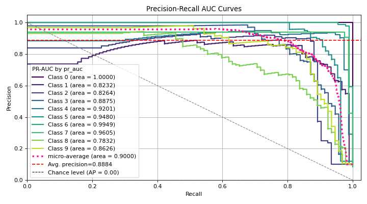